This 1st version of the DEswan vignette briefly describes how to use this package to analyze the links between a quantitative trait (qt) and high dimensional datasets such as -omics data. Here we apply DEswan to the data generated by Lehallier et al. (https://www.biorxiv.org/content/10.1101/751115v1).

Install development version from GitHub

# library(devtools)
# devtools::install_github("lehallib/DEswan",build_vignettes = T)

Data description

This aging proteomic dataset was generated using SOMAscan. Lehallier et al. measured 1305 plasma proteins from 171 individuals ranged from young adults to centenarians from 4 different cohorts.

# devtools::install("../DEswan")
library("DEswan")
head(agingplasmaproteome[,1:5])
#>   Age    Sex Cohort Feature_1 Feature_2
#> 1 107 Female PRIN09     3.249     2.850
#> 2 105   Male PRIN09     3.105     2.801
#> 3 106 Female PRIN09     3.149     2.841
#> 4 106   Male PRIN09     3.205     2.876
#> 5 105   Male PRIN09     3.159     2.961
#> 6 105   Male PRIN09     3.337     2.860

The first three column are demographics and samples’ characteristics. Columns 4:1308 are levels of plasma proteins in a log10 scale.

Age is the qt of interest and Sex and Cohort are covariates we want to include in the analysis


# distribution of qt
hist(agingplasmaproteome[,1],main="qt distribution",xlab="Age (years)")

# covariates
table(agingplasmaproteome[,2])
#> 
#> Female   Male 
#>     87     84
table(agingplasmaproteome[,3])
#> 
#>    GEHA  PRIN06  PRIN09 Seattle 
#>      26      51      24      70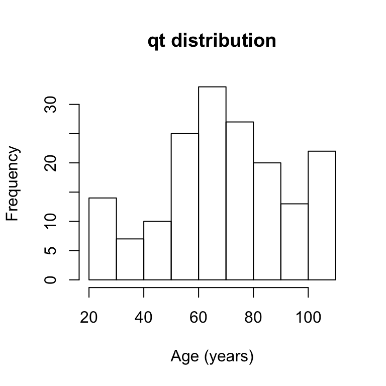

DEswan

To run DEswan we call the function DEswan(). DEswan() takes 5 arguments (3 are optional):

⋅⋅* data.df: a data Frame - columns are variables and rows are samples (same order as qt and covariates)

⋅⋅* qt: a Vector - quantitative trait for DE-SWAN (same order as data.df and covariates)

⋅⋅* window.center: an optional Vector - window centers. Default is quantile(qt, probs = seq(.1,.9,.1))

⋅⋅* buckets.size: an optional Numeric - size of each bucket. Default is set to (max(range(qt))-min(range(qt)))/2

⋅⋅* covariates: a data Frame. Columns are variables and rows are samples (same order as qt and covariates)


x=cor(agingplasmaproteome[,1],agingplasmaproteome[,-c(1:3)])
head(agingplasmaproteome[,1:5])
#>   Age    Sex Cohort Feature_1 Feature_2
#> 1 107 Female PRIN09     3.249     2.850
#> 2 105   Male PRIN09     3.105     2.801
#> 3 106 Female PRIN09     3.149     2.841
#> 4 106   Male PRIN09     3.205     2.876
#> 5 105   Male PRIN09     3.159     2.961
#> 6 105   Male PRIN09     3.337     2.860
start_time <- Sys.time()
# res.DEswan=DEswan(data.df = agingplasmaproteome[,-c(1:3)],
res.DEswan=DEswan(data.df = agingplasmaproteome[,3+c(which(colnames(x) %in% colnames(x)[abs(x)>.5]))],
                  qt = agingplasmaproteome[,1],
                  window.center = seq(35,95,10),
                  buckets.size = 20,
                  covariates = agingplasmaproteome[,c(2:3)])
#> [1] "window.center  1/7"
#> [1] "window.center  2/7"
#> [1] "window.center  3/7"
#> [1] "window.center  4/7"
#> [1] "window.center  5/7"
#> [1] "window.center  6/7"
#> [1] "window.center  7/7"
end_time <- Sys.time()
end_time-start_time
#> Time difference of 5.328683 secs

The output of is a list of 2 data.frames: p = pvalues of qT and covariates for each variable and each window.center coefficients = coefficients of qT and covariates for each variable and each window.center

head(res.DEswan$p)
#>     variable window.center factor       pvalue
#> 1 Feature_19            35     qt 0.5982000400
#> 2 Feature_19            35    Sex 0.5392278397
#> 3 Feature_19            35 Cohort 0.9942942114
#> 4 Feature_54            35     qt 0.0457508523
#> 5 Feature_54            35    Sex 0.0001776826
#> 6 Feature_54            35 Cohort 0.0331861758
head(res.DEswan$coeff)
#>                            variable window.center        factor
#> (Intercept)              Feature_19            35   (Intercept)
#> qt.tmp1                  Feature_19            35            qt
#> covariates$SexMale       Feature_19            35       SexMale
#> covariates$CohortSeattle Feature_19            35 CohortSeattle
#> (Intercept)1             Feature_54            35   (Intercept)
#> qt.tmp11                 Feature_54            35            qt
#>                            coefficient
#> (Intercept)               3.6228803069
#> qt.tmp1                  -0.0194542199
#> covariates$SexMale        0.0218608696
#> covariates$CohortSeattle  0.0004792839
#> (Intercept)1              3.6366547315
#> qt.tmp11                  0.0434974425

Note on computational time

Increasing the resolution of DEswan (more values in “window.center” vector) will provide more detailed results but will require additional computational time. Computational time also depends on the number of features included in the analysis.

Next releases of DEswan will focus on decreasing computational time.

Reshape DEswan results

DEswan outputs are in long format. Reshaping the results to wide format helps the exploration of the statistics produces by DEswan

res.DEswan.wide.p=reshape.DEswan(res.DEswan,parameter = 1,factor = "qt")
head(res.DEswan.wide.p[,1:5])
#>       variable        X35        X45        X55          X65
#> 1  Feature_100 0.07590300 0.29734451 0.86476347 2.929219e-04
#> 2 Feature_1032 0.87131724 0.48797672 0.04809311 8.216263e-02
#> 3 Feature_1056 0.44283629 0.47567400 0.05464477 5.982463e-05
#> 4 Feature_1058 0.62735503 0.64697045 0.39293953 5.509108e-02
#> 5 Feature_1062 0.06621829 0.09694809 0.86923229 1.476878e-01
#> 6 Feature_1064 0.93689325 0.87715881 0.41877198 2.094534e-01

Pvalues adjustment

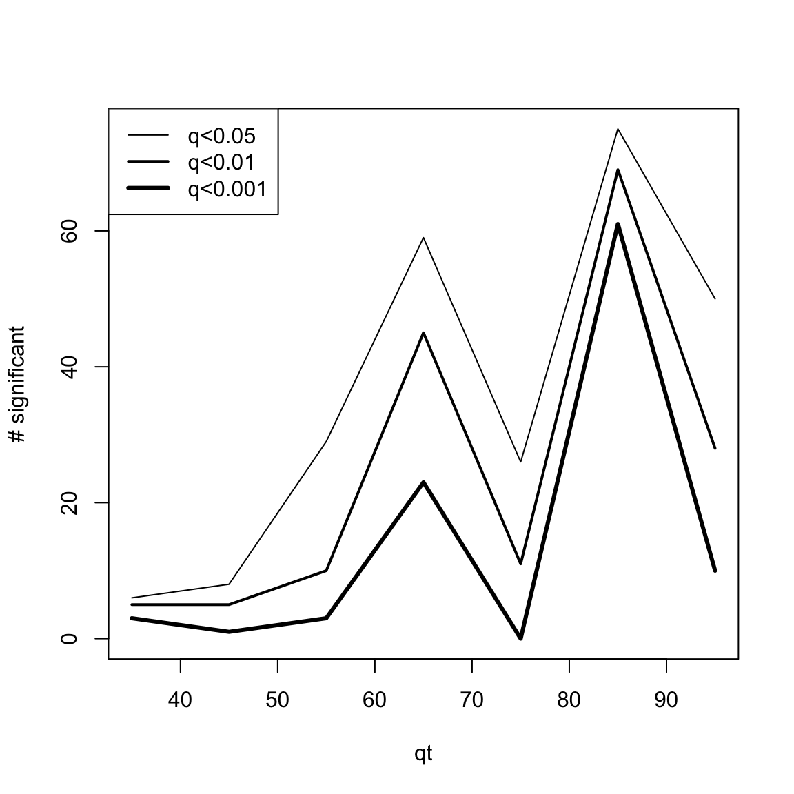
Methods for dealing with multiple testing frequently call for adjusting α in some way. The Bonferroni correction is one simple way to take this into account; adjusting the false discovery rate using the Benjamini-Hochberg procedure is a more powerful method.

res.DEswan.wide.q=q.DEswan(res.DEswan.wide.p,method="BH")
head(res.DEswan.wide.q[,1:5])
#>       variable       X35       X45       X55          X65
#> 1  Feature_100 0.3715252 0.5867818 0.9178181 0.0010896693
#> 2 Feature_1032 0.9568731 0.7439645 0.1177016 0.1076214765
#> 3 Feature_1056 0.7487959 0.7439645 0.1209991 0.0003272759
#> 4 Feature_1058 0.8174135 0.8232951 0.4834008 0.0764697147
#> 5 Feature_1062 0.3421278 0.3467759 0.9178181 0.1716870179
#> 6 Feature_1064 0.9568731 0.8964370 0.4914348 0.2318948642

Calculate and plot the number of significant variables

One simple way to visualize DEswan results is to count the number of significant variables for each window.center tested.

# head(res.DEswan.wide.p[,1:5])
res.DEswan.wide.p.signif=nsignif.DEswan(res.DEswan.wide.p)
toPlot=res.DEswan.wide.p.signif[1:3,]
x=as.numeric(gsub("X","",colnames(toPlot)))
plot(1, type = "n", xlim=c(min(x,na.rm=T),max(x,na.rm=T)),ylim=c(0,max(toPlot,na.rm=T)),ylab="# significant",xlab="qt")
for(i in 1:nrow(toPlot)){
  lines(x,
        toPlot[i,],type='l',lwd=i)
}
legend("topleft",legend = paste("p<",rownames(toPlot),sep=""),lwd=c(1,2,3))


# head(res.DEswan.wide.q[,1:5])
res.DEswan.wide.q.signif=nsignif.DEswan(res.DEswan.wide.q)
toPlot=res.DEswan.wide.q.signif[1:3,]
x=as.numeric(gsub("X","",colnames(toPlot)))
plot(1, type = "n", xlim=c(min(x,na.rm=T),max(x,na.rm=T)),ylim=c(0,max(toPlot,na.rm=T)),ylab="# significant",xlab="qt")
for(i in 1:nrow(toPlot)){
  lines(x,
        toPlot[i,],type='l',lwd=i)
}
legend("topleft",legend = paste("q<",rownames(toPlot),sep=""),lwd=c(1,2,3))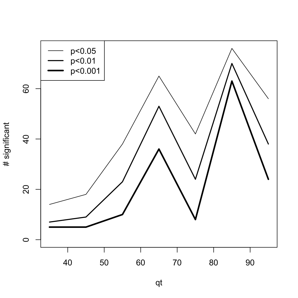

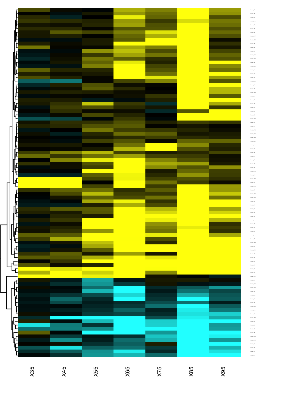
Heatmap of changes during aging

The best way to identify when and how the features are changing in the qt space is to generate a heatmap of the signed effects.



res.DEswan.wide.coeff=reshape.DEswan(res.DEswan,parameter = 2,factor = "qt")
toHeatmap=sign(res.DEswan.wide.coeff[,-1])*-log10(res.DEswan.wide.p[,-1])
rownames(toHeatmap)<-res.DEswan.wide.coeff$variable

pairs.breaks <- seq(-3, 3, by=0.01)
mycol <- gplots::colorpanel(n=length(pairs.breaks)-1,low="cyan",mid="black",high="yellow")

# display the colorbar
# image(z = matrix(1:100, ncol = 1),col = mycol,xaxt = "n",yaxt = "n")

gplots::heatmap.2(as.matrix(toHeatmap),
                       cexRow=.1,cexCol=.7,
                       trace="none",
                       dendrogram="row",
                       breaks=pairs.breaks, 
                       col=mycol, 
                       Rowv=T,key=F,
                       Colv=F,
                       lhei=c(0.2,10),
                       lwid=c(.2,3)
)

Covariates analysis

Similar analysis can be generated for each covariates. Here we show how sex affect the plasma proteome during aging



res.DEswan.wide.p.covar1=reshape.DEswan(res.DEswan,parameter = 1,factor = "Sex")
res.DEswan.wide.coeff.covar1=reshape.DEswan(res.DEswan,parameter = 2,factor = "SexMale")

toHeatmap=sign(res.DEswan.wide.coeff[,-1])*-log10(res.DEswan.wide.p[,-1])
rownames(toHeatmap)<-res.DEswan.wide.coeff$variable

pairs.breaks <- seq(-3, 3, by=0.01)
mycol <- gplots::colorpanel(n=length(pairs.breaks)-1,low="cyan",mid="black",high="yellow")

# display the colorbar
# image(z = matrix(1:100, ncol = 1),col = mycol,xaxt = "n",yaxt = "n")

gplots::heatmap.2(as.matrix(toHeatmap),
                       cexRow=.1,cexCol=.7,
                       trace="none",
                       dendrogram="both",
                       breaks=pairs.breaks, 
                       col=mycol, 
                       Rowv=T,key=F,
                       Colv=F,
                       lhei=c(0.2,10),
                       lwid=c(.2,3)
)
#> Warning in gplots::heatmap.2(as.matrix(toHeatmap), cexRow = 0.1, cexCol
#> = 0.7, : Discrepancy: Colv is FALSE, while dendrogram is `both'. Omitting
#> column dendogram.

DEswan vignette

Benoit Lehallier

2019-09-25